Mass Harmonics: The Gaia DR4 Prediction Set

Eight prospective prediction pathways, nine measurable outcomes, and one scale-invariant acceleration law spanning stellar binaries, the Milky Way, and the Solar System

We've traveled through neuronal architecture with MICrONS, molecular closure with wwPDB, galactic structure with Rubin, fundamental matter with ICHEP, and gravitational-wave propagation and compact-object boundaries with LIGO-Virgo-KAGRA.

Now, for the final prediction paper in Mass Harmonics Volume I, we arrive at something particularly compelling.

What if the gravitational behavior of two widely separated stars and the gravitational behavior of an entire galaxy are expressions of exactly the same physical boundary relationship?

And what if we can test both using measurements released by the same astronomical mission?

That is the central idea behind the Gaia DR4 prediction set.

The paper predicts that a single acceleration scale, derived from the ψₘ substrate rather than fitted independently to galaxies or binary stars, will determine where the familiar inverse-square gravitational response transitions toward the outer-boundary behavior described by Mass Harmonics.

But it goes further. It specifies the transition distance, the velocity relationship, the direction of the additional acceleration, the behavior of stellar streams, and the absence of that low-acceleration enhancement in the high-acceleration Solar System.

I retrieved the full original document through EZ23+:

MH_PREDICTION_07_Gaia_DR4_2026-12-02_Mass_Harmonics_Governed.md

Prospective release December 2, 2026

Prediction pathways 8

Final measurable readouts 9

Source contact 1,210 lines, complete

EZ23+ verified Git blob: 75201f83db9eb133dad1e2c65b88d09603578e3a.

The distinction between eight pathways and nine readouts is deliberate. The first pathway predicts both a universal transition acceleration and its mass-dependent physical separation.

This paper was completed before the targeted Gaia release. Its results are therefore presented here as prospective theoretical predictions, not as experimentally confirmed Gaia DR4 findings.

Gaia spacecraft against the Milky WayImage: ESA · opens original

SECTION 011. What is Gaia, and why is DR4 so important?#

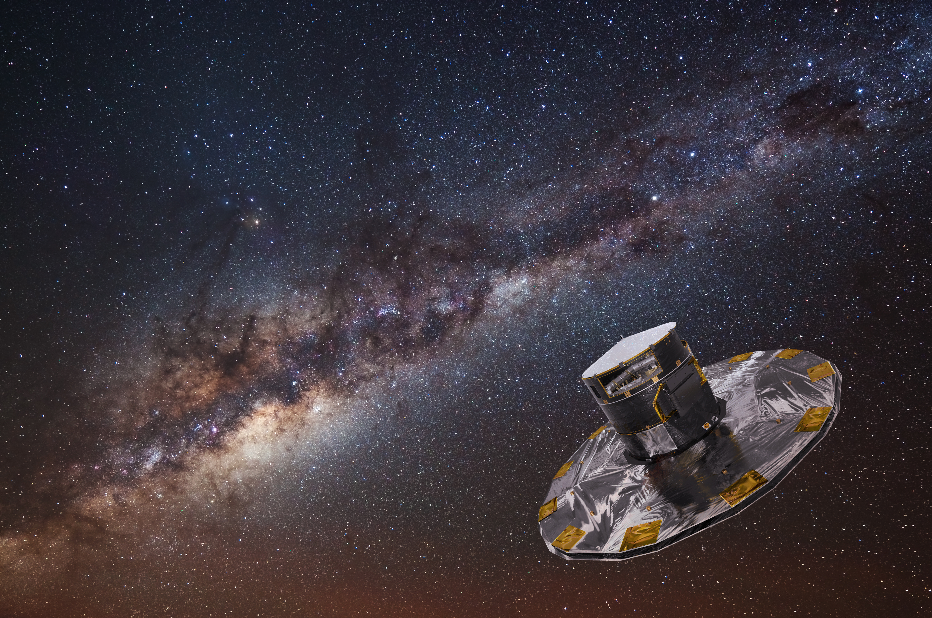
The entity["other","Gaia","European Space Agency stellar astrometry mission"] mission was designed to produce an extraordinarily precise map of the stars and other objects in and around our galaxy.

Instead of simply photographing stars, Gaia measures their positions, distances, apparent motions, brightness, and, for suitable sources, radial velocities.

That allows astronomers to reconstruct how stars move through three-dimensional space.

Consider two stars in the night sky.

From a single image, they might appear near each other.

But they could actually lie hundreds of light-years apart.

Gaia's distance and motion measurements help distinguish chance alignments from genuine physical companions.

This is especially important for wide binary stars.

What are wide binaries?

A binary system contains two stars gravitationally associated with one another.

Some binary stars orbit very close together.

Others are separated by thousands or tens of thousands of astronomical units.

Close binary

The mutual acceleration is comparatively strong.

Wide binary

At large separation, the mutual acceleration becomes extremely small.

Why does that matter?

Because the separation between two stars determines the strength of their familiar inverse-square mutual acceleration:

g_N=\frac{G_NM_T}{r^2}

where $M_T$ is their combined mass and $r$ their separation.

Increase the separation, and the acceleration decreases with the square of the distance.

A sufficiently wide binary therefore offers a way to investigate gravitational behavior at extremely low accelerations.

What Gaia DR4 contributes

The source describes Gaia DR4 as a major expansion of the observational terrain, using approximately 66 months of observations and expected to include billions of sources and numerous product families.

Relevant products include improved astrometry, epoch measurements, radial velocities, non-single-star solutions, stellar parameters, and Solar-System measurements.

These allow multiple kinds of investigation:

Wide binary motion

Determine how pairs of stars behave as their mutual accelerations become exceptionally small.

Milky Way dynamics

Examine how stars move through the Galactic disk and how their motion relates to the distribution of ordinary matter.

Stellar streams

Investigate long, coherent structures of stars that retain information about gravitational influences across their trajectories.

Solar-System controls

Examine high-acceleration orbital motion where the source predicts that the low-acceleration enhancement should not appear.

The profound opportunity is not merely that Gaia measures many stars.

It is that the mission supplies observational information relevant to different bounded systems across very different physical scales.

And Mass Harmonics predicts that those systems should retain the same underlying acceleration relationships when expressed through the appropriate dimensionless ratios.

SECTION 022. The causal spine of the entire paper#

The Gaia paper is built on a compact and explicit physical derivation.

It begins with the Mass Harmonics substrate, carries its closure law to cosmological scale, and then transports the resulting acceleration relationship into stellar and Galactic systems.

The governing Master Field Equation is:

\frac{1}{vₓ^2}\ddot{\psi}_m - Z(\psi_m)\nabla^2\psi_m - \frac{8K\psi_m}{\omega^2}|\nabla\psi_m|^2 = S(\rho)

with:

Z(\psi_m)=1+\frac{8K\psi_m}{\omega^2}

The source identifies the acceleration relationship:

\boxed{ a_0=\frac{cH_0}{2\pi} }

and its outer-boundary expression:

\boxed{ g_{\mathrm{MH}}\approx\sqrt{g_Na_0} }

The familiar inverse-square expression remains:

g_N=\frac{G_NM}{r^2}

The resulting circular-motion relation is:

\boxed{ v^4=G_NMa_0 }

These relationships also appeared in the Rubin prediction paper.

The important difference is where they are now being tested.

Rubin principally investigates galaxies and their lensing signatures.

Gaia transports the same relations into wide binaries, the Milky Way's stellar motions, and Solar-System controls.

That cross-scale transport is a prospective extension of the canonical galactic Mass Harmonics branch, rather than a separate binary-specific derivation appearing verbatim in the Monograph.

Illustration of different radial dependencies; not observed Gaia or Rubin data.

SECTION 033. The source-locked numerical acceleration scale#

The Gaia paper uses the pre-release numerical Hubble input:

H_0=70\ \mathrm{km\,s^{-1}\,Mpc^{-1}}

Converting into inverse seconds:

H_0=2.268545502611056\times10^{-18}\ \mathrm{s^{-1}}

The source then evaluates:

a_0=\frac{cH_0}{2\pi}

giving:

\boxed{ a_0=1.082401360239200\times10^{-10}\ \mathrm{m/s^2} }

That is an extraordinarily small acceleration.

For perspective, the familiar acceleration associated with gravity near Earth's surface is about 9.8 meters per second squared.

The Mass Harmonics transition acceleration is roughly ninety billion times smaller.

It becomes relevant in systems whose gravitational influence has weakened across enormous separations.

One dimensionless comparison for all systems

The paper defines two quantities:

\boxed{X=\frac{g_N}{a_0}}

\boxed{Y=\frac{g_{\mathrm{obs}}}{a_0}}

These are dimensionless.

They express an observed acceleration relative to the same underlying acceleration anchor.

In the high-acceleration interior:

X\gg1\quad\Rightarrow\quad Y\approx X

In the low-acceleration outer-boundary limit:

X\ll1\quad\Rightarrow\quad Y\approx\sqrt X

Equivalently:

\boxed{ \frac{Y^2}{X}\rightarrow1 }

in the deep-boundary limit.

This relationship is the organizing principle of the Gaia paper.

The physical masses and separations can vary enormously. But once expressed using $X$ and $Y$, the source predicts that the relevant low-acceleration systems must follow the same asymptotic relationship.

That is the meaning of scale invariance being tested here.

SECTION 044. Prediction G1: Wide binaries should transition at one universal acceleration, not one fixed distance#

G1 · Universal low-acceleration transition and mass-scaled separation

This first prediction is particularly elegant because it produces a distance from an acceleration condition.

Step 1: Identify the two physical limits

The familiar interior relation is:

\[Y=X\]

The outer-boundary relation is:

Y=\sqrt X

At the nonzero point where these two expressions meet:

X=\sqrt X

Squaring:

\[X^2=X\]

Therefore:

\[X(X-1)=0\]

The nonzero transition occurs at:

\boxed{X=1}

Since:

X=\frac{g_N}{a_0}

the transition condition becomes:

\boxed{g_N=a_0}

This is the physical boundary anchor.

What does that mean?

The paper does not predict that every binary star system changes behavior at, for example, 7,000 astronomical units.

It predicts that the transition occurs when the system's own mutual acceleration reaches the same universal acceleration value.

More massive binary systems can remain above that acceleration threshold at greater separations.

Less massive systems reach it sooner.

Step 2: Derive the transition separation

For two stars whose combined mass is $M_T$:

g_N=\frac{G_NM_T}{r^2}

Set:

\frac{G_NM_T}{r_t^2}=a_0

Rearrange:

r_t^2=\frac{G_NM_T}{a_0}

Therefore:

\boxed{ r_t=\sqrt{\frac{G_NM_T}{a_0}} }

Substituting the universal acceleration:

\boxed{ r_t=\sqrt{\frac{2\pi G_NM_T}{cH_0}} }

The central scaling relationship is:

\boxed{r_t\propto M_T^{1/2}}

The actual mass-dependent predictions

Using the source's acceleration anchor:

Combined stellar mass	Predicted transition separation
0.2 $M_\odot$	3,310.23 AU
0.5 $M_\odot$	5,233.93 AU
1.0 $M_\odot$	7,401.89 AU
2.0 $M_\odot$	10,467.86 AU
5.0 $M_\odot$	16,551.14 AU
10.0 $M_\odot$	23,406.84 AU

Notice the progression.

A binary with one solar mass reaches the transition near 7,402 AU.

A binary with four times that mass would reach it at twice that separation.

The law is mass-dependent, but the acceleration condition remains identical.

Step 3: Translate the prediction into Gaia's measurements

Gaia observes angular positions and motions.

It does not directly report an invisible physical boundary surrounding every stellar pair.

For a system at distance $d_{\mathrm{pc}}$ parsecs, the predicted angular separation is:

\theta_t= \frac{7401.893067}{d_{\mathrm{pc}}} \sqrt{\frac{M_T}{M_\odot}} \ \mathrm{arcsec}

For a one-solar-mass binary:

Distance from Earth	Predicted angular transition
25 pc	296.08 arcsec
50 pc	148.04 arcsec
100 pc	74.02 arcsec
200 pc	37.01 arcsec
500 pc	14.80 arcsec

These are observational projections of the same physical transition distance.

An important complication: the Milky Way's tidal field

A wide binary is not isolated from the rest of the galaxy.

Both stars experience the Milky Way's gravitational influence.

The common contribution acting on both stars largely cancels when studying their relative acceleration.

But the differential galactic field across their separation does not cancel.

The paper explicitly identifies this tidal contribution:

\mathbf g_{\mathrm{rel,measured}} = \mathbf g_{\mathrm{binary}} + \mathbf T_{\mathrm{Gal}}\mathbf r + \mathbf g_{\mathrm{perturb}} + \mathbf g_{\mathrm{error}}

The binary acceleration must therefore be recovered after accounting for the Galactic tidal tensor and identifiable local perturbations.

Otherwise, an apparent low-acceleration signal might actually reflect the environment surrounding the pair.

What would falsify G1?

The source specifies several distinct contradictions.

A fixed transition distance independent of binary mass would contradict the prediction.

So would transition accelerations that vary systematically with stellar mass or population after physical controls.

A failure of the square-root mass scaling would also contradict it.

And a clean eligible sample showing no continuous transition near $g_N=a_0$ would challenge the proposed boundary behavior.

G1's decisive claim is not simply that wide binaries may behave differently at large separations. It is that their transition must occur at a universal acceleration whose physical radius scales with the square root of total stellar mass.

SECTION 055. Prediction G2: Widely separated binaries should approach a mass-dependent velocity asymptote#

G2 · Deep-boundary velocity and acceleration invariants

The first prediction tells us where a binary should enter its boundary transition.

The second tells us how its motion should behave after entering the low-acceleration domain.

This is a powerful distinction.

Under a simple inverse-square gravitational model, circular orbital speed decreases as separation increases:

v_N=\sqrt{\frac{G_NM_T}{r}}

Consequently:

v_N\propto r^{-1/2}

Double the separation and the circular speed decreases.

The Mass Harmonics deep-boundary law produces a different result.

Step 1: Start from the outer-boundary acceleration

g_{\mathrm{MH}}=\sqrt{g_Na_0}

Substitute:

g_N=\frac{G_NM_T}{r^2}

Then:

g_{\mathrm{MH}}= \sqrt{\frac{G_NM_Ta_0}{r^2}}

Therefore:

g_{\mathrm{MH}}= \frac{\sqrt{G_NM_Ta_0}}{r}

Step 2: Apply circular relative-motion kinematics

For an approximately circular binary:

g_{\mathrm{MH}}=\frac{v_{\mathrm{rel}}^2}{r}

Equating the two expressions:

\frac{v_{\mathrm{rel}}^2}{r} = \frac{\sqrt{G_NM_Ta_0}}{r}

Cancel the common radius:

v_{\mathrm{rel}}^2=\sqrt{G_NM_Ta_0}

Square again:

\boxed{ v_{\mathrm{rel}}^4=G_NM_Ta_0 }

Therefore:

\boxed{ v_{\mathrm{rel},\infty}=(G_NM_Ta_0)^{1/4} }

The result is remarkable because the separation has disappeared from the deep-boundary expression.

Instead, the limiting circular relative velocity depends on the fourth root of the binary's total mass.

The predicted velocities

Combined mass	Deep-boundary relative speed
0.2 $M_\odot$	0.231519 km/s
0.5 $M_\odot$	0.291119 km/s
1.0 $M_\odot$	0.346201 km/s
2.0 $M_\odot$	0.411705 km/s
5.0 $M_\odot$	0.517691 km/s
10.0 $M_\odot$	0.615642 km/s

Step 3: Convert the prediction into a dimensionless invariant

The paper defines:

\boxed{ W_{\mathrm{binary}} = \frac{v_{\mathrm{rel}}^4}{G_NM_Ta_0} }

In the deep-boundary limit:

\boxed{W_{\mathrm{binary}}\rightarrow1}

This is the key observational result.

It allows systems with very different component masses to be compared through the same normalized quantity.

Why orbital eccentricity matters

Here the source makes an important distinction.

The circular-speed expression cannot be applied blindly to an eccentric orbit at an arbitrary phase.

A star moving along an elongated orbit continually changes both its distance from its companion and its instantaneous velocity.

Using that velocity as though the orbit were circular would create a category error.

For eccentric binaries, the source prioritizes direct relative acceleration:

\boxed{ \frac{g_{\mathrm{obs}}^2}{g_Na_0}\rightarrow1 }

in the deep-boundary limit.

That test can preserve the physical acceleration relationship without forcing an instantaneous velocity into circular-orbit kinematics.

What would falsify G2?

Clean low-acceleration binaries whose speeds continue the inverse-square circular decline, whose limiting speeds fail the fourth-root mass relationship, or whose direct acceleration invariant does not approach one would contradict the prediction.

The paper also requires checking whether residual differences correlate with metallicity, stellar age, sky position, or other population properties.

G2 predicts a specific asymptotic response. It does not merely predict that wide binaries have slightly larger velocities than expected.

SECTION 066. Prediction G3: Binary accelerations should form one continuous universal curve#

G3 · Continuous transition between interior and outer-boundary behavior

G1 specifies the location of the transition.

G2 specifies the outer behavior.

G3 asks whether every eligible binary population traces the same continuous physical progression between the two.

This matters because a physical substrate governed by one continuous equation should not require unrelated binary-specific force laws merely because different stars have different masses.

The two fixed limits

Recall:

X=\frac{g_N}{a_0}

Y=\frac{g_{\mathrm{obs}}}{a_0}

The high-acceleration limit is:

Y\approx X

The deep-boundary limit is:

Y\approx\sqrt X

The source predicts a single continuous, monotonic transition:

\boxed{Y=F_{\mathrm{MH}}(X)}

It deliberately does not insert an empirical interpolation formula.

The detailed intermediate shape is left to the full local MFE solution and subsequent comparison with observational terrain.

That limitation is important: G3 fixes the endpoints, transition scale, continuity, and mass-independence, but it does not supply a complete numerical transition curve at every intermediate $X$.

Explore the two source-fixed limits

Acceleration position $X=g_N/a_0$

Slider

Current value unavailable.

Range: -3 to 3

Step: 0.1

Normalized $X$

Interior $Y=X$

Boundary $Y=\sqrt X$

The slider compares the two mathematical limits. It does not invent an intermediate Mass Harmonics solution.

What does it mean for different binary populations to collapse onto one curve?

Imagine studying low-mass red-dwarf pairs and more massive stellar pairs.

Their physical transition separations are different.

Their relative velocities are different.

Their luminosities, temperatures, and observational uncertainties are different.

But if the source's universality claim is correct, converting every system into $X$ and $Y$ should remove those irrelevant scale differences.

The resulting relationships should converge onto the same continuous physical curve.

This is called data collapse.

What would falsify G3?

If the different mass populations require independent transition accelerations, different dimensionless amplitudes, or incompatible interpolation behavior, the asserted universality breaks.

Likewise, a discontinuity not associated with a genuine change in physical boundary conditions would contradict the source.

A particularly important result would be a consistent low-acceleration discrepancy whose magnitude depends on stellar population even after the physical controls.

That would require more than simply declaring a universal curve.

SECTION 077. Prediction G4: The additional binary acceleration should point radially, with no universal torque#

G4 · Scalar-gradient alignment and zero-torque signature

This is a geometrical prediction about the direction of acceleration.

The previous predictions mostly concern magnitudes.

But force has direction as well as strength.

Mass Harmonics proposes that the relevant additional acceleration originates from a scalar-gradient contribution:

\boxed{ \mathbf g_{\mathrm{Giboney}} = -\nabla\left(\frac{\psi_m^2}{\omega}\right) }

For an isolated approximately symmetric two-body coherence structure, the source predicts that the additional acceleration acts along the line connecting the components.

Visualizing the distinction

Predicted central correction

Not a universal source term

Direction diagrams are conceptual. Environmental tides and local perturbations can still generate transverse accelerations.

Step 1: Express the radial condition

The source predicts:

\Delta\mathbf g_{\mathrm{MH}} \parallel-\hat{\mathbf r}

That means the additional low-acceleration contribution follows the separation axis, pointing toward the other component in the attractive branch.

Step 2: Calculate torque

Torque is:

\boldsymbol\tau=\mathbf r\times\mathbf F

For a central force:

\mathbf F=-|\mathbf F|\hat{\mathbf r}

Therefore:

\boldsymbol\tau= \mathbf r\times(-|\mathbf F|\hat{\mathbf r})

Because the vectors are parallel:

\boxed{\boldsymbol\tau=0}

So the additional force changes radial acceleration without introducing a universal sideways twist.

Why is this useful?

If an apparent low-acceleration anomaly systematically points in a particular sky direction, depends on orbital handedness, or appears primarily perpendicular to the separation axis, it would be difficult to reconcile with the declared central-gradient relationship.

The paper does not prohibit actual transverse perturbations.

Galactic tides, close encounters, hidden companions, and observational errors can produce them.

What it excludes is a universal non-central correction attributed to the same bounded two-body substrate structure.

What would falsify G4?

A reproducible residual that is predominantly transverse after physical corrections, possesses a preferred celestial direction, or changes sign with orbital handedness would contradict this prediction.

The direction of the anomaly is therefore an additional independent constraint, not merely another way of fitting its magnitude.

SECTION 088. Prediction G5: The Milky Way's outer disk should obey the same baryonic boundary law#

G5 · Galactic circular-speed invariant

Now the paper changes scale dramatically.

We have been examining pairs of stars separated by thousands of astronomical units.

The fifth prediction examines the orbital motion of stars across the Milky Way, a system spanning tens of thousands of light-years.

Yet the governing physical relationship remains unchanged.

Step 1: Begin with the source's galactic boundary law

\[v_c^4=G_NM_ba_0\]

Here $v_c$ is the circular speed and $M_b$ is the enclosed baryonic mass relevant to the outer boundary.

When the enclosed baryonic mass has substantially converged:

v_c\rightarrow\text{constant}

Therefore:

\boxed{ \frac{d\ln v_c}{d\ln R}\rightarrow0 }

The predicted outer rotation curve becomes approximately flat.

What does a flat rotation curve mean?

Imagine a collection of planets orbiting a star.

Farther planets generally move more slowly because the gravitational acceleration decreases with distance.

Now consider stars moving around a galaxy.

The familiar observation that many galaxies have comparatively flat outer rotation curves is one of the principal reasons astronomers infer additional gravitating mass.

Mass Harmonics assigns the extended acceleration response to the ψₘ substrate.

The same mathematical relation that generated the wide-binary velocity asymptote now generates the outer Galactic circular-speed relationship.

Step 2: Construct the dimensionless Milky Way invariant

The source defines:

Enclosed baryonic mass	Predicted outer circular speed
$4\times10^{10}M_\odot$	154.83 km/s
$5\times10^{10}M_\odot$	163.71 km/s
$6\times10^{10}M_\odot$	171.34 km/s
$10^{11}M_\odot$	194.68 km/s

Observable	Source-fixed requirement
Universal transition acceleration	$g_N=a_0$
Mass-scaled transition distance	$r_t\propto M_T^{1/2}$
Deep-boundary binary motion	$v_{\mathrm{rel}}^4=G_NM_Ta_0$
Binary acceleration invariant	$g_{\mathrm{obs}}^2/(g_Na_0)\to1$
Direction of additional acceleration	Central, radial; zero universal torque
Milky Way outer boundary	$v_c^4=G_NM_ba_0$
Stellar-stream residuals	Spatially coherent and gradient-aligned
Binary-Galaxy cross-scale identity	$W_{\mathrm{binary}}\to1$ and $W_{\mathrm{MW}}\to1$
Solar-System high-acceleration control	$Y\approx X$; no deep-boundary enhancement

Gaia DR4

Mass Harmonics: The Gaia DR4 Prediction Set

SECTION 011. What is Gaia, and why is DR4 so important?#

What are wide binaries?

What Gaia DR4 contributes

SECTION 022. The causal spine of the entire paper#

SECTION 033. The source-locked numerical acceleration scale#

One dimensionless comparison for all systems

SECTION 044. Prediction G1: Wide binaries should transition at one universal acceleration, not one fixed distance#

Step 1: Identify the two physical limits

What does that mean?

Step 2: Derive the transition separation

The actual mass-dependent predictions

Step 3: Translate the prediction into Gaia's measurements

An important complication: the Milky Way's tidal field

What would falsify G1?

SECTION 055. Prediction G2: Widely separated binaries should approach a mass-dependent velocity asymptote#

Step 1: Start from the outer-boundary acceleration

Step 2: Apply circular relative-motion kinematics

The predicted velocities

Step 3: Convert the prediction into a dimensionless invariant

Why orbital eccentricity matters

What would falsify G2?

SECTION 066. Prediction G3: Binary accelerations should form one continuous universal curve#

The two fixed limits

Explore the two source-fixed limits

What does it mean for different binary populations to collapse onto one curve?

What would falsify G3?

SECTION 077. Prediction G4: The additional binary acceleration should point radially, with no universal torque#

Visualizing the distinction

Step 1: Express the radial condition

Step 2: Calculate torque

Why is this useful?

What would falsify G4?

SECTION 088. Prediction G5: The Milky Way's outer disk should obey the same baryonic boundary law#

Step 1: Begin with the source's galactic boundary law

What does a flat rotation curve mean?

Step 2: Construct the dimensionless Milky Way invariant

Step 3: The actual numerical predictions

Why the baryonic mass must be independently reconstructed

Different stellar populations must recover the same underlying field

What would falsify G5?

Why G5 matters

SECTION 099. Prediction G6: Stellar streams should reveal a smooth, coherent residual field#

Step 1: Identify the predicted residual

Step 2: Translate that into a spatial prediction

Coherent field versus local disturbance

Does this exclude ordinary perturbations?

What would falsify G6?

Why this is important

SECTION 1010. Prediction G7: Wide binaries and the Milky Way must recover the same invariant#

The two invariants

Why this is more demanding than G2 or G5 individually

The acceleration-collapse requirement

What would falsify G7?

Why G7 is the centerpiece

SECTION 1111. Prediction G8: The Solar System should remain a high-acceleration null control#

Step 1: Identify the Solar-System domain

Step 2: The expected residual

Why is a null control so valuable?

But Solar-System motion contains many other forces

What would falsify G8?

Why the final prediction completes the set

SECTION 1212. The complete Gaia DR4 prediction matrix#

SECTION 1313. The observational safeguards#

SECTION 1414. What makes the December 2026 release especially interesting?#

SECTION 1515. What would constitute a particularly significant result?#

SECTION 1616. The wider significance of Volume I#

The Gaia paper in everyday language

You have reached the end of Volume I